Comp The Player: Classifying NBA Players
With the expansion in popularity of NBA basketball over the years, an enormous amount of data is now being produced from game to game. This no longer is limited to simple counting stats like points, rebounds, and assists – we can now ask questions like: “How many times did Klay Thompson dribble the ball before shooting in the 3rd quarter? How many miles did he run on defense? How many times did he shoot from beyond 24 feet?”
I recently spent some time scraping such data from the web in order to do some exploratory analysis on NBA basketball players (see my Github for code). One of the simplest questions we can ask is: what defines a player? Not in terms of production or value, but stylistically, how does a player play?
In my explorations, I have found that it is difficult to use unsupervised methods such as k-means clustering to define style of play, because the number of features and groups to use becomes highly arbitrary with so many different ways to play.
Therefore, I constructed a player classification model, with the target labels being the veteran players themselves. Such a model allows us to find the best “comp” for, say, rookie players who are frequently scouted by NBA front offices searching for cheap talent. With this motivation in mind, let’s see how such a model can be built.
A Word About Random Forest Classification
A common tool used for regression and classification is the decision tree, which is a tree-like structure beginning with a root. From this starting node, which includes the entire sample, the algorithm decides which of the input features provides the most information for differentiating the sample data (i.e. player-seasons). The algorithm then splits the data on this feature.
The formula for information gain provided by a new feature is given by the difference between the entropy for the current node, , and weighted sum of the entropies of the nodes resulting from splitting the data on the new feature, :
The entropy of is simply calculated from each (the probability/proportion of the th class):
The entropy is weighted by number of samples in each resultant node, preventing an insignificant node from dominating the entropy.
The algorithm repeats this process for each node, each time computing the information gain for the remaining input features. In this way, a tree is “grown” in descending order of information gain. For a nice, detailed explanation broken down using examples, see this article.
Now, if we can grow a tree, why not grow a forest? A random forest is a collection of many decision trees, which is highly advantageous for many problems. Each tree is a random sub-sample of the input training data (a sampling technique known as bootstrapping), and each tree uses a subset of input features. A vote is tallied from each tree’s prediction in order to determine the overall prediction, essentially averaging over all estimators. This entire process is known as bagging, short for bootstrap aggregation.
Below is a cartoon from this article by Rosaria Silipo and Kathrin Melcher.
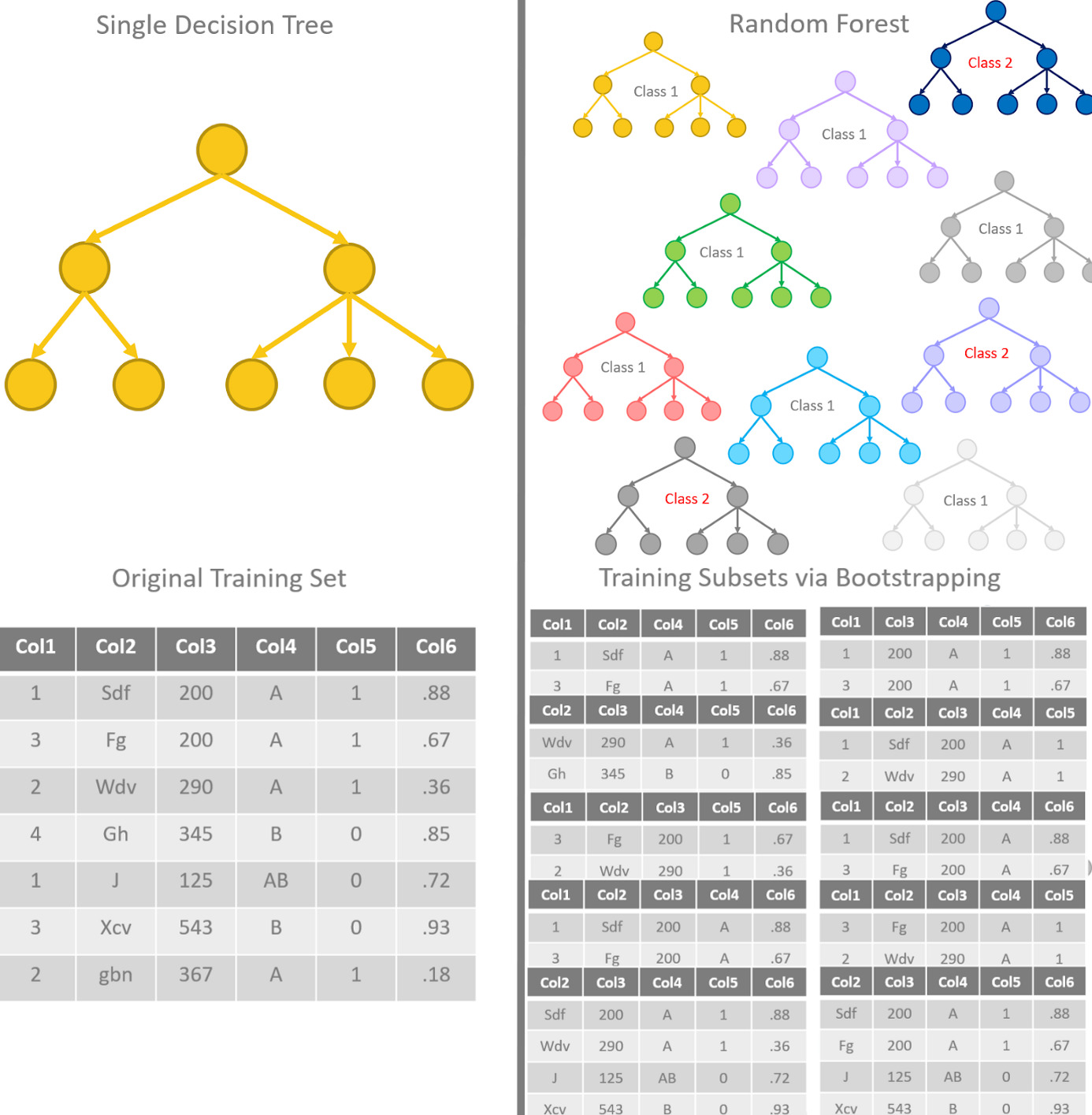
The strengths of this algorithm are that it can handle missing values, it automatically accounts for relative feature importance, and it avoids overfitting by cancelling out the large variance associated with each tree.
As we will see, our model will consist of 181 output labels, which is the number of veteran players who played for the last 4 complete NBA seasons (2016-2019). Not only are there many labels, but there are also many input features to differentiate style of play. What’s more, we only have 3 samples per label to work with if we leave out one season as a test dataset.
For all these reasons, the Random Forest model is the ideal candidate for performing player classification.
Feature Selection
Through some exploratory data analysis which I will not thoroughly detail here, combined with some basketball logic and intuition, the input features below were selected for the random forest classification (RFC).
Shown is a Python snippet which displays the relevant features in a Pandas dataframe, which was the result of data scraping from a variety of NBA data sources.
# Specify which dataframe columns to use as model features
feature_list = ['height', 'weight', 'FG_FREQ_05FT', 'FG_FREQ_59FT', 'FG_FREQ_1014FT', 'FG_FREQ_1519FT', 'FG_FREQ_2024FT', 'FG_FREQ_GT24FT', 'FG_FREQ_CANDS', 'FTR', 'ASTR', 'TOR', 'ORR', 'DRR', 'BLK_PH', 'STL_PH', 'DFGP_PG']

# Display the dataframe with selected features
pd.set_option('display.max_columns', 13)
df[['name'] + feature_list]
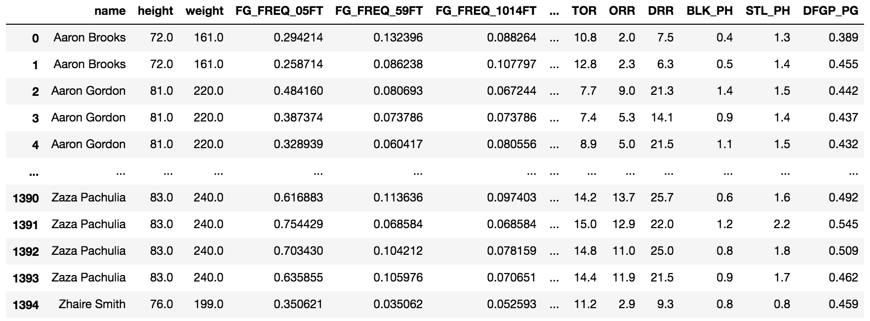
These stats can be summarized as follows:
- ‘height’ – player height in inches
- ‘weight’ – player weight in lbs
- ‘FG_FREQ_05FT’ – percentage of shots from 0-5 ft. from the basket
- ‘FG_FREQ_59FT’ – percentage of shots from 5-9 ft. from the basket
- ‘FG_FREQ_1014FT’ – percentage of shots from 10-14 ft. from the basket
- ‘FG_FREQ_1519FT’ – percentage of shots from 15-19 ft. from the basket
- ‘FG_FREQ_2024FT’ – percentage of shots from 20-24 ft. from the basket
- ‘FG_FREQ_GT24FT’ – percentage of shots from > 24 ft. from the basket
- ‘FG_FREQ_CANDS’ – percentage of shots that are catch-and-shoot (no dribbles)
- ‘FTR’ – free throw rate
- ‘ASTR’ – assist rate
- ‘TOR’ – turnover rate
- ‘ORR’ – offensive rebounding rate
- ‘DRR’ – defensive rebounding rate
- ‘BLK_PH’ – shot blocks (per 100 possessions)
- ‘STL_PH’ – steals (per 100 possessions)
- ‘DFGP_PG’ – defensive/opponent field goal percentage
Note that height and weight are hardly “play-style” attributes, but rather physical attributes. They are still important since strict lines between player positions, e.g. point guards, shooting guards, centers, etc., are becoming increasingly blurred in the modern NBA, but a player’s size still determines how a player is utilized.
The offensive stats are relatively self-explanatory; we largely differentiate a player by where on the floor they take their shots, how often they draw fouls, and how often they make plays or rebound the ball.
A player’s defense is more difficult to quantify, however the opponent’s defensive field goal percentage is included to account for man-on-man defense in addition to a player’s blocks and steals.
It is worth noting that this list is neither exhaustive nor completely optimized. These resulted in decent accuracy, however there are a variety of unused additional stats that would be interesting to leverage. For example, I have also scraped play-type stats: how often does a player score on pick-and-rolls? Put-backs? Isolation plays? However, this would greatly increase the number of features and statistical interactions have not been thoroughly studied.
Creating a Random Forest Model
To create the RFC model, we first separate the input data into veterans and rookies. Here, veterans are all players who played in each season from 2016-2019, while rookies only played in the 2019 season.
I then divide the veteran dataset into a training set (3 seasons) and a testing set (the 2019 season), as out-of-sample testing will be used to calculate the unbiased accuracy of our model. I also separate the training and testing datasets into input features and output labels (the player names).
# Create separate dataframes for established players and rookies
df_vets = df[df["name"].isin(df["name"].value_counts()[df["name"].value_counts() == 4].index)]
df_train = df_vets[df_vets.year < 2019]
df_test = df_vets[df_vets.year == 2019]

df_rooks = df[df["name"].isin(df["name"].value_counts()[df["name"].value_counts() == 1].index)]
df_rooks = df_rooks[df_rooks.year == 2019]

# Create input features and target labels (player names) for test data
test_labels = df_test[["name"]]
test_features = df_test[feature_list]

# Create matching training dataset using only veterans who are still in the NBA
# (and thus have available training data)
train_labels = df_train[["name"]]
train_features = df_train[feature_list]
In order to properly fit our input training data, it is also a good idea to scale the input features to unit variance and subtract their means. This is a good habit when training machine learning algorithms to aid in model convergence and avoid feature biases.
# Scale features which will be used in model fitting
# (for both training and testing datasets)
scale_train = StandardScaler().fit(train_features)
train_features = scale_train.transform(train_features)
test_features = scale_train.transform(test_features)
A comprehensive grid search is performed on the various hyperparameters of the RandomForestClassifier in scikit-learn, using the GridSearchCV k-fold cross validation method. This is actually quite time intensive, but worth it given the large number of features and output labels.
# Perform a comprehensive grid search to optimize parameters for Random Forest classification
n_estimators = [100, 500, 1000, 2000, 5000]
max_depth = [5, 15, 30]
min_samples_split = [2, 10, 100]
min_samples_leaf = [1, 5, 10]

param_grid = {'n_estimators': n_estimators, 'max_depth' : max_depth, 'min_samples_split' : min_samples_split, 'min_samples_leaf' : min_samples_leaf}
grid_search = GridSearchCV(RandomForestClassifier(random_state = 1), param_grid, cv=3)
grid_search.fit(train_features, train_labels.values.ravel())
grid_search.best_params_
print('Optimized hyperparameters:', grid_search.best_params_)

rfc = RandomForestClassifier(
    n_estimators=grid_search.best_params_['n_estimators'],
    max_depth=grid_search.best_params_['max_depth'],
    min_samples_split=grid_search.best_params_['min_samples_split'],
    min_samples_leaf=grid_search.best_params_['min_samples_leaf'] )

rfc.fit(train_features, train_labels.values.ravel())
Once the hyperparameters are optimized, we fit the training data to create our RFC model.
The model is then run on our test dataset (the 2019 dataset for each veteran player). The accuracy here is then simply the fraction of veterans that were properly identified with themselves (from previous seasons).
# Run the classifier model on the test data
y_pred = rfc.predict(test_features)
print("Classified veteran players with an accuracy of", np.sum(test_labels.name.values==y_pred)*100./(len(y_pred)*1.), "%")
Output:
Classified veteran players with an accuracy of 92.81767955801105 %
As we can see, we correctly predict that veteran players are themselves with great accuracy, despite season-to-season variation. This is not far-fetched, since we are providing the player’s physical attributes, however given fluctuations in the other stats this is still a solid result.
Results for Rookies in the 2019 Season
Once we have a trained and tested model, we can ideally run the classifier on any player not used in the training data to find their best player “comp”.
It is worth noting: this is not a comparison of production or value. Aside from defensive FGP, the features used in the model are rate or frequency stats meant to characterize play style rather than performance.
# Format rookie dataset for input into the classifier and
# attempt to classify rookies by their most similar veteran counterpart
pred_labels = df_rooks[["name"]]
pred_features = df_rooks[feature_list]

pred_features = scale_train.transform(pred_features)
rook_pred = rfc.predict(pred_features)

for i,pred in enumerate(rook_pred):
    print("Predicted that Rookie", pred_labels.name.values[i], "is similar to Player:", pred)
Output:
Predicted that Rookie Aaron Holiday is similar to Player: Isaiah Canaan
Predicted that Rookie Alfonzo McKinnie is similar to Player: JaMychal Green
Predicted that Rookie Boban Marjanovic is similar to Player: Jusuf Nurkic
Predicted that Rookie Bonzie Colson is similar to Player: PJ Tucker
Predicted that Rookie Brandon Sampson is similar to Player: Jordan Clarkson
Predicted that Rookie Bruce Brown is similar to Player: Tyreke Evans
Predicted that Rookie Cameron Reynolds is similar to Player: Wesley Matthews
Predicted that Rookie Chandler Hutchison is similar to Player: Justise Winslow
Predicted that Rookie Cheick Diallo is similar to Player: Taj Gibson
Predicted that Rookie Christian Wood is similar to Player: Karl-Anthony Towns
Predicted that Rookie DJ Wilson is similar to Player: Markieff Morris
Predicted that Rookie Daniel Hamilton is similar to Player: D'Angelo Russell
Predicted that Rookie Daryl Macon is similar to Player: Kemba Walker
Predicted that Rookie De'Aaron Fox is similar to Player: Jeff Teague
Predicted that Rookie De'Anthony Melton is similar to Player: Tyus Jones
Predicted that Rookie Deandre Ayton is similar to Player: Alex Len
Predicted that Rookie Deng Adel is similar to Player: Klay Thompson
Predicted that Rookie Derrick White is similar to Player: Cory Joseph
Predicted that Rookie Devin Robinson is similar to Player: Giannis Antetokounmpo
Predicted that Rookie Deyonta Davis is similar to Player: Cody Zeller
Predicted that Rookie Donte DiVincenzo is similar to Player: Eric Gordon
Predicted that Rookie Duncan Robinson is similar to Player: Kyle Korver
Predicted that Rookie Dwayne Bacon is similar to Player: Tobias Harris
Predicted that Rookie Furkan Korkmaz is similar to Player: Terrence Ross
Predicted that Rookie Gary Clark is similar to Player: Kyle Korver
Predicted that Rookie Henry Ellenson is similar to Player: Frank Kaminsky
Predicted that Rookie Isaiah Briscoe is similar to Player: TJ McConnell
Predicted that Rookie Ivan Rabb is similar to Player: Taj Gibson
Predicted that Rookie Jake Layman is similar to Player: Aaron Gordon
Predicted that Rookie Jalen Brunson is similar to Player: Tyus Jones
Predicted that Rookie James Nunnally is similar to Player: Tony Snell
Predicted that Rookie Jaron Blossomgame is similar to Player: Tobias Harris
Predicted that Rookie Jaylen Adams is similar to Player: Tyus Jones
Predicted that Rookie Jemerrio Jones is similar to Player: Rajon Rondo
Predicted that Rookie Jevon Carter is similar to Player: Raymond Felton
Predicted that Rookie John Jenkins is similar to Player: JJ Redick
Predicted that Rookie Johnathan Williams is similar to Player: Kenneth Faried
Predicted that Rookie Jonah Bolden is similar to Player: Nikola Mirotic
Predicted that Rookie Josh Jackson is similar to Player: Andrew Wiggins
Predicted that Rookie Josh Okogie is similar to Player: Victor Oladipo
Predicted that Rookie Julian Washburn is similar to Player: Nicolas Batum
Predicted that Rookie Kadeem Allen is similar to Player: TJ McConnell
Predicted that Rookie Keita Bates-Diop is similar to Player: Jeff Green
Predicted that Rookie Kenrich Williams is similar to Player: Thabo Sefolosha
Predicted that Rookie Kevin Huerter is similar to Player: D'Angelo Russell
Predicted that Rookie Khem Birch is similar to Player: Kenneth Faried
Predicted that Rookie Landry Shamet is similar to Player: Marco Belinelli
Predicted that Rookie Luka Doncic is similar to Player: James Harden
Predicted that Rookie Malik Beasley is similar to Player: Courtney Lee
Predicted that Rookie Malik Monk is similar to Player: Langston Galloway
Predicted that Rookie Mikal Bridges is similar to Player: Thabo Sefolosha
Predicted that Rookie Miles Bridges is similar to Player: Justise Winslow
Predicted that Rookie Monte Morris is similar to Player: Dennis Schroder
Predicted that Rookie Moritz Wagner is similar to Player: Kelly Olynyk
Predicted that Rookie Rawle Alkins is similar to Player: JaMychal Green
Predicted that Rookie Ray Spalding is similar to Player: John Henson
Predicted that Rookie Rodions Kurucs is similar to Player: Maurice Harkless
Predicted that Rookie Ryan Broekhoff is similar to Player: Kyle Korver
Predicted that Rookie Semi Ojeleye is similar to Player: Stanley Johnson
Predicted that Rookie Shai Gilgeous-Alexander is similar to Player: Shaun Livingston
Predicted that Rookie Shake Milton is similar to Player: Josh Richardson
Predicted that Rookie Terrance Ferguson is similar to Player: Justin Holiday
Predicted that Rookie Theo Pinson is similar to Player: Vince Carter
Predicted that Rookie Thomas Bryant is similar to Player: DeMarcus Cousins
Predicted that Rookie Trae Young is similar to Player: Jeff Teague
Predicted that Rookie Tyler Dorsey is similar to Player: Zach LaVine
Predicted that Rookie Yuta Watanabe is similar to Player: Evan Turner
Predicted that Rookie Zach Collins is similar to Player: Karl-Anthony Towns
Predicted that Rookie Zhaire Smith is similar to Player: Damian Lillard
Shown above are the predictions for each 2019 rookie. Just to get a sense that these comparisons are sensible, let’s dive into an example.
An Example Comparison
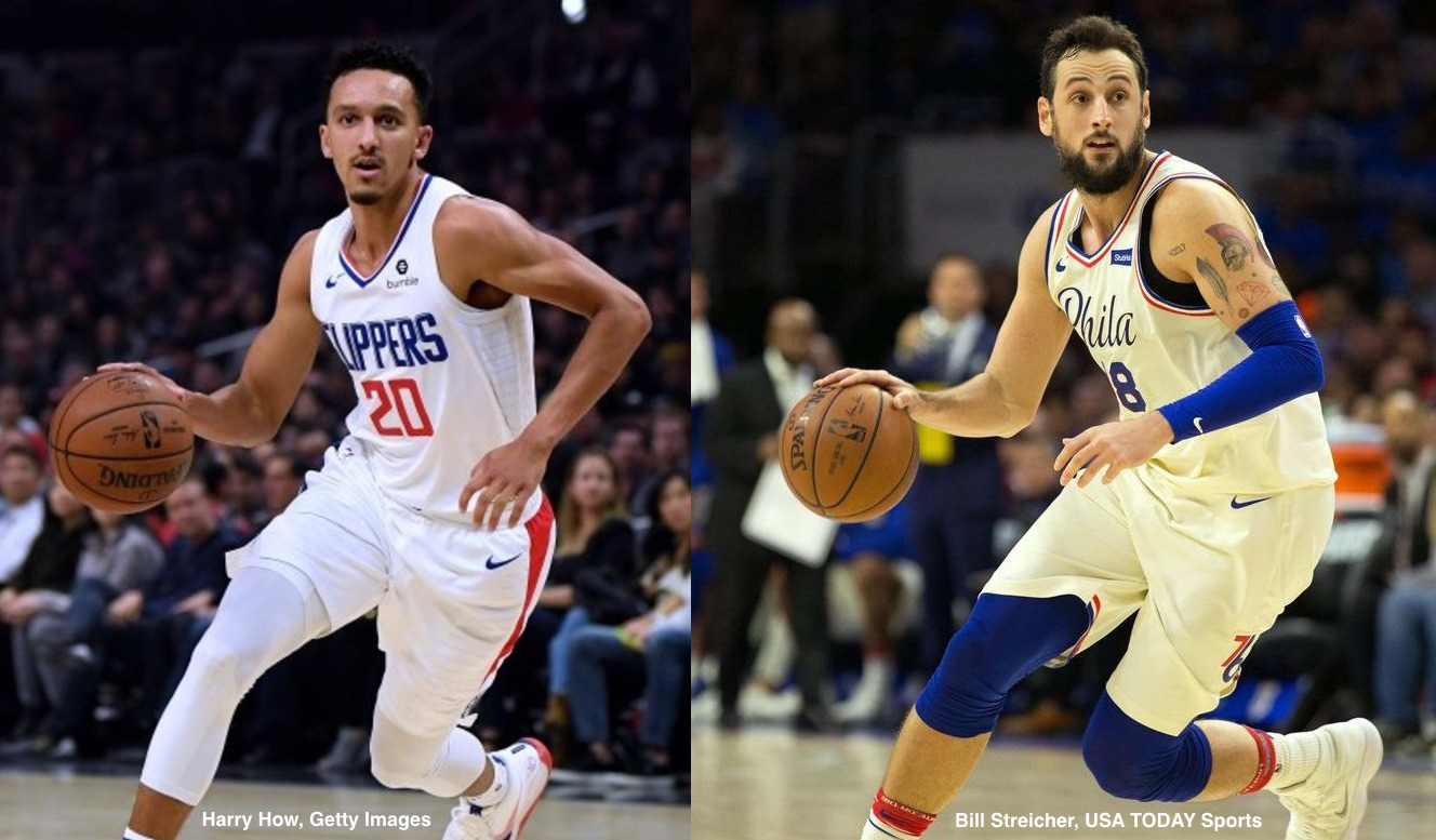
Our classifier algorithm found Landry Shamet and Marco Belinelli to have matching play styles. Shamet came into the league with low expectations, but was a pleasant surprise and made an early impact as a shooter on the L.A. Clippers. Belinelli is a veteran player also known for his exceptional shooting skills off the bench.
We can simply plot these players in a number of feature spaces and examine how similar they really are.
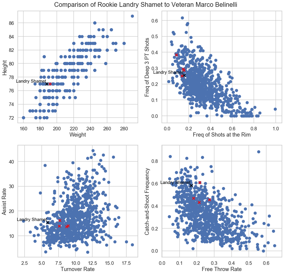
As we can see, they are indeed very similar. They are both lanky shooting guards who like to shoot deep 3-pointers. They are both limited play-makers who get around half their shots from catch-and-shoot action (i.e. without dribbling before the shot). Belinelli tended to shoot more free throws over the last few years, but this could merely indicate that he is older and more experienced with drawing fouls.
Why is this useful?
NBA team front offices and scouting teams spend an enormous amount of time scouting and evaluating players. Scouts fly all over the world to watch players live, they organize workouts to perform the “eye test”, and the media often portrays a player in a light that effectively skews general perception.
In short, biases are a part of the evaluation system. This algorithm is a method for providing a direct comparison with veteran players who are successful enough to have found a role in the league.
Not only does this classification tool provide an unbiased label that may not have been considered by glancing at a box score, it also allows front offices to seek out cheap talent to fill a specific role. If a rebuilding team is looking for a young backup catch-and-shoot guard who plays tenacious defense, this algorithm may indicate which players are closer to Klay Thompson than James Harden.