An RAPM Model to Assess NBA Players
If you are like me, you watch NBA basketball games with a healthy mixture of enthusiasm for the game and skepticism of the media-driven narratives. In the last several years, I noticed a wide variety of advanced stats being thrown around by fans and media members alike, seemingly to justify their biased conclusions about players with highly subjective analysis. What’s more, these stats are frequently used as definitive arguments for end-of-season awards, such as MVP.
You hear things like: “Player X is clearly superior to Player Y because he ranks higher in categories A, B, and C.” Inevitably, you hear the response: “We all know stats A, B, and C don’t necessarily translate to winning games!”
Even with such advanced stats, there is sometimes widespread disagreement about a player’s impact or value. There are multiple issues at play with these stats:
- They are heavily influenced by simple box score stats, some of which have arguable relevance to a player’s overall impact.
- Many of them are generated using historical data, biasing more recent evaluations.
- They are often taken out of applicable context (perhaps due to lack of transparency).
Below, I will discuss my own attempt to “objectively” assess player impact by creating a RAPM model and compare those results with existing stats. However, some words are in order about the existing landscape of advanced stats.
Player Impact Metrics
To get a broad survey of existing methodologies, let’s take a look at just some of the most popular advanced player stats that exist (follow the links to get a more detailed description):
- Hollinger’s Player Efficiency Rating (PER)
- Plus-Minus/Adjusted Plus-Minus/RAPM
- Box Plus-Minus (BPM), by Daniel Myers
- ESPN’s Real Plus-Minus (RPM), by Jeremias Engelmann
- Player Impact Plus-Minus (PIPM), by Jacob Goldstein of BBall Index
Such player impact stats can be roughly categorized as follows: purely box score–based stats, Statistical Plus-Minus (SPM) models, and actual Plus-Minus models (usually based on RAPM).
PER belongs to the first category. It is an all-in-one stat which uses a fixed formula to give a measure of player production from simple box score stats (e.g. points, rebounds, assists, turnovers, steals, blocks, personal fouls). While PER succeeds in combining box score stats into a single number, there are plenty of criticisms surrounding its methodology and biases.
BPM falls into the category of SPM models. While it is also based on box score stats, it is a regression against historical RAPM datasets to determine the coefficients which weight each feature (RAPM, a variant of plus-minus, will be discussed below). In other words, SPM models are linear estimators of RAPM.
It is easy to see why box score–based stats are limited; this can’t possibly encompass the entirety of a player’s impact! Consider some of the things not taken into account by simple box score stats:
- Man-on-man and help defense
- Screen-setting to open up shooters
- Player gravity (drawing the defense)
- Floor spacing (threat of deep 3-point shooting)
- Quality of passing (not the same as the rate of assists or turnovers)
- Intangibles (e.g. leadership, communication on defense, etc.)
We would like to capture a player’s intangibles, or anything that is not shown by the box score. Plus-Minus based stats may be used for this purpose, since they are based purely on overall team success when the player is on the floor. The advanced stats we have not yet discussed, RPM and PIPM, are both based on RAPM, which is a successor of Plus-Minus. Let’s take a deeper look at what this means, and why this technique is so prominent in basketball analytics.
What is Regularized Adjusted Plus-Minus?
The original Plus-Minus stat is simply the point differential a team experiences when a player is on the floor (i.e. points scored by the team minus points scored against the team). However, it is well-established that this metric is deceptive, since a player surrounded by highly skilled teammates will have an inflated Plus-Minus.
To answer this, an Adjusted Plus-Minus (APM) was created to account for these effects. This essentially means creating a matrix of n possessions by m players involved in all those possessions. We can set entries to if the player is on offense in the possession, if on defense, and if not on the floor. We can then formulate a matrix equation to solve for the coefficients that give the resulting point differentials :
We then approximate the coefficients by solving for the least-squares solution to the matrix equation. This yields values which actually represent the player contributions, removing the effect of teammates and opposing players.
These coefficients are the player APM values. However, because of multicollinearity, the results have enormous variance. Luckily, there is a statistical technique for dealing with this very issue: L2 regularization, or ridge regression. This is a well-known method for penalizing outlier values back to the central value, to reduce variance at the expense of bias.
Ridge regression is performed by modifying the least squares formulation with a diagonal perturbation matrix :
The value is a model hyperparameter that must be tuned to stabilize the coefficients. Note that in the limit that , we recover least squares; in the limit , shrinks to .
In this case, the resulting coefficients are the RAPM values, or the Regularized Adjusted Plus-Minus for each player. To be clear, these values are not absolute points added. This regularization technique results in coefficients that are scaled by a factor dependent on . The RAPM values should therefore be taken as a relative stat, or a differential contribution.
Circling back, how do our advanced stats incorporate RAPM? SPM models like BPM use RAPM strictly as an input to find the model coefficients. RPM and PIPM, on the other hand, are essentially “enhanced” RAPM models which use Bayesian priors to constrain the coefficients based on a fit to historical RAPM datasets. As we will discuss, this puts a potentially biased emphasis on box score stats.
Harvesting Matchups from Play-by-Play Data
In order to create my own RAPM model, I constructed a matrix as explained above, as well as the point differential resulting from each row (each matchup stint). I performed the following procedure:
- Scrape play-by-play data from all NBA games over several seasons
- Parse the PBP data into stints, or matchups between player lineups (that may last a number of possessions)
- Calculate the point differential resulting from each stint, and from that the array (which is actually the plus-minus per 100 possessions)
- Create a matrix with stints (rows) and NBA players (columns)
To scrape the data, I used a Selenium web driver in Python to parse play-by-play data from NBA.com. These tables track the score and provide raw text data for analyzing the content of each play. In addition, the starting lineup for each quarter was fetched separately, allowing for player rotations to be tracked throughout a game. This is crucial for monitoring which lineups are out on the floor at any time.
The full scraping and wrangling codes can be found at my Github.

Once we’ve isolated each matchup, we can parse the lineups into individual players for the home and away teams. Since we are taking the results of a stint, rather than single possessions, each team has been on both offense and defense. Therefore, we give home team players a matrix entry of , away team players an entry of , and players not on the floor an entry of . We then take to be the home team plus-minus per 100 possessions.
This can be done with a Python function as shown below:
def GenerateMatchupMatrix(df, player_list):
    matchup_plus_minus = []
    rapm_matrix = np.zeros(shape=(len(df),len(player_list)), dtype=float)
    idx=0

    for index, stint in df.iterrows():
        if idx%100 == 0:
            sys.stdout.write("\rOn Stint %i..." % (idx+1))
            sys.stdout.flush()

        matchup_plus_minus.append(stint.ht_pm_ph)

        f_ht_p, f_allp_ind, f_htl_ind = np.intersect1d(player_list, stint.ht_lineup.split(','), return_indices=True)
        rapm_matrix[idx,f_allp_ind] = 1
        f_vt_p, f_allp_ind, f_vtl_ind = np.intersect1d(player_list, stint.vt_lineup.split(','), return_indices=True)
        rapm_matrix[idx,f_allp_ind] = -1

        idx += 1

    print('\n Finished!')
    return rapm_matrix, matchup_plus_minus
Once we have and , we can build a ridge regression model to estimate the coefficients .
Developing a Ridge Regression Model
In order to optimize our ridge regression model, we will use the matchup matrix and matchup point differential as our training data and perform k-fold cross-validation to use the training data itself for validation. This is important, since we have only 3 seasons of NBA data (2017-2019).
In Python, we use the Ridge model from scikit-learn along with the GridSearchCV method to perform cross-validation on a comprehensive set of parameters (Note: in the Ridge model).
x_train = rapm_matrix
y_train = matchup_plus_minus

ridge_reg = Ridge()
alphas = [1, 10, 50, 100, 500, 1000, 1500, 2000, 3000, 5000]
param_grid = {'alpha': alphas}
grid_search = GridSearchCV(ridge_reg, param_grid, cv=3)
grid_search.fit(x_train, y_train)

print('Optimized hyperparameters:', grid_search.best_params_)

Output:
>> Optimized hyperparameters: {'alpha': 1500}
While k-fold cross-validation is typically used to set , we can also make sense of our choice by plotting the calculated RAPM as a function of .
It is clear that the values for small are highly unstable, as certain players experience a lot of variance. We can see that for our optimized parameter, the best– and worst–RAPM players are stable and begin to converge to the mean.
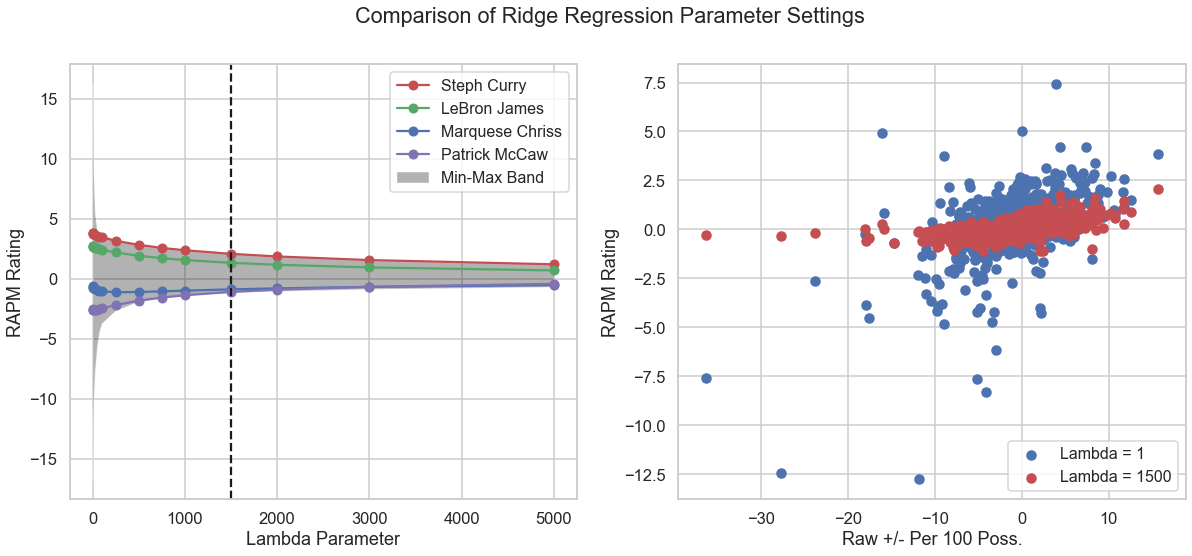
We therefore tune our hyperparameter with some degree of confidence. It is important to point out that our typical notion of out-of-sample model testing is compromised here; season-to-season variation in player performance is an unavoidable reality (for numerous reasons), and this model is meant to produce a descriptive stat rather than a predictive one. But more on that later.
Evaluating Player RAPM Ratings
Let’s take a look at how various players fare in RAPM.
Along with play-by-play data, individual stats were scraped for NBA players, including net rating, BPM, and RPM (again, see my Github). Note that net rating is actually just the player’s raw plus-minus per 100 possessions, which doesn’t take into account the caliber of a player’s supporting cast.
Below, we see the top 10 and bottom 10 players in RAPM (of players averaging minutes per game), along with these other metrics.
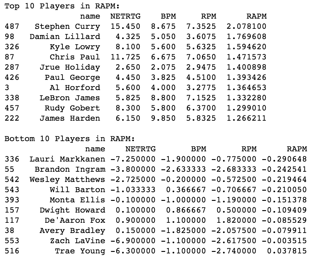
Stephen Curry has league-leading RAPM over the last 3 years, which is not outlandish given that he is a transformative player of this era. It is more interesting that the top 5 players are all guards – smaller players, 3 of whom are considered excellent 2-way players and all of whom can shoot 3-pointers and make plays for others. Notice also that some players, especially Damian Lillard and Jrue Holiday, are highly underrated by ESPN’s RPM.
If you are a basketball fan, I know you may scoff at the fact that Jrue Holiday is ranked “better” than LeBron James over a 3 year span. My response to this: the reasons you have for assuming LeBron James would have a better regular season RAPM may be very biased. If you take away LeBron James’s:
- Usage rate and time spent with the ball in his hands
- Previous accomplishments (prior to 2017)
- Playoff performances (we are only looking at the regular season)
- Media narratives
- “Flashiness”
it is not so far-fetched. Think about it: Jrue Holiday is young, plays both ends of the floor, is an efficient scorer and play-maker, and has largely played a complementary role without an outstanding supporting cast. I’m not here to argue that Jrue Holiday is better than LeBron James in general, however the purpose of this exercise is to remove biased assumptions.
On the other hand, the players with the worst RAPM tend to be either aging, inexperienced, or considered lazy on at least one end of the floor. For instance, Trae Young is a rookie considered to be one of the worst defenders in the league.
An important note: I am by no means claiming these RAPM ratings are perfect or the end-all-be-all. These will of course have error, but still may provide some interesting unbiased perspective when evaluating players.
Comparing with Other Advanced Stats
To understand what we’ve calculated better, and how it relates to existing metrics, we can examine correlations with a variety of box score and advanced stats.
A useful tool for doing this is to make a Pearson correlation heatmap. This allows us to examine relationships between a large number of features and potentially informs us on what dependencies to examine further.
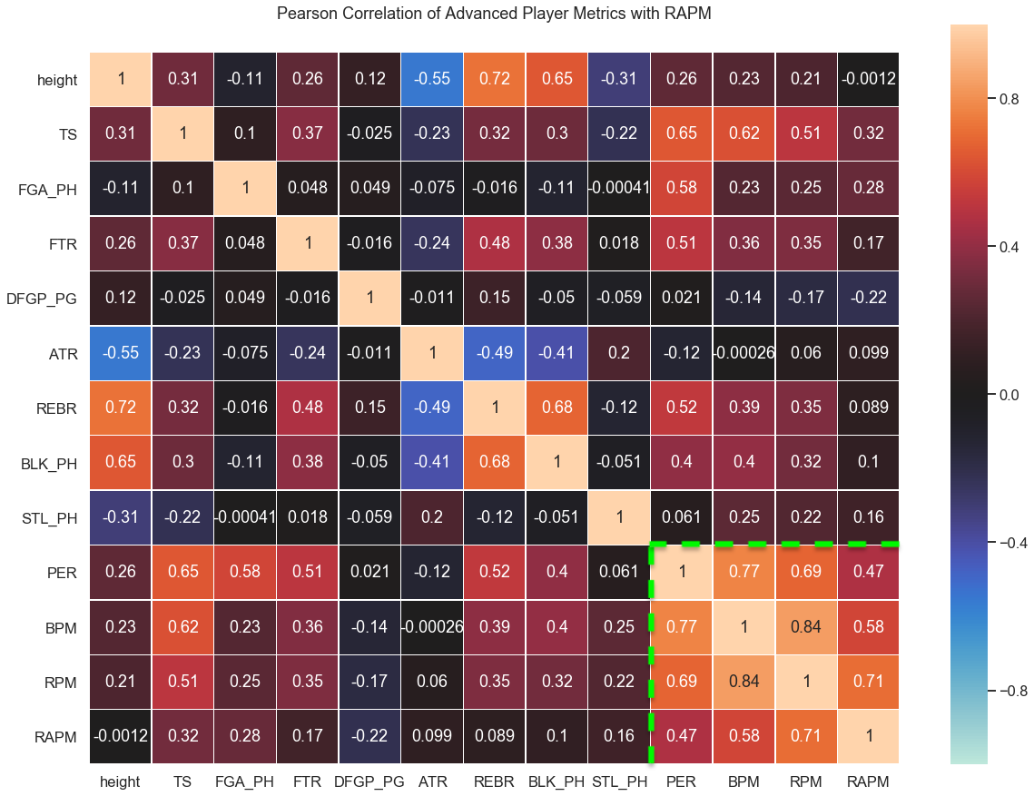
Shown in the matrix above are correlations between various player statistics averaged over the 2017-2019 seasons, including the previously discussed PER, BPM, RPM, and RAPM (within the green lines). The other abbreviated stats are: true shooting %, field goal attempts per 100 possessions, free throw rate, opponent field goal %, assist-to-turnover ratio, rebound rate, blocks per 100 poss., and steals per 100 poss.
We can summarize some interesting points from this table:
- PER has a much higher correlation with field goal attempts than the other stats (it rewards players who simply take more shots)
- PER, BPM, and RPM all have a slight correlation with player height, while RAPM is completely uncorrelated with height
- PER, BPM, and RPM give much more weight to rebounds and blocks than RAPM (but interestingly, not steals)
- RAPM is the most anticorrelated with opponent field goal %, which serves as a proxy for man-on-man defense (which is hard to quantify)
- RAPM is less correlated with true shooting % than the other stats, though this is also true for the free throw rate (and free throws factor in to true shooting)
- PER and RPM are more correlated with BPM than RAPM
Taking all these observations together, it is reasonable to conclude that
- Other advanced stats appear to favor big men, including stats that are typical for big men (e.g. rebounds and blocks)
- ESPN’s RPM, one of the most popular and quoted advanced stats, appears to be highly dependent on box score stats
The explanation for this is that the RPM methodology uses box score priors calculated from a historical 15-year RAPM dataset (a cursory overview of such a technique is given in this article about PIPM). These Bayesian priors are then used in the ridge regression to constrain the range of for various players, thus pre-estimating their value using their box score stats. While these priors are proprietary and not publicly available, it appears that the box score component is significant (and even such factors as height and age are directly included).
Conclusions
At the beginning of this article, I provided 3 criticisms of current player impact metrics. Let’s discuss how my RAPM ratings address each:
- Box score dependence – there is none, not even assumed box score priors.
- Historical bias – RAPM in this context is calculated from only a 3-year dataset, providing sufficient statistics without biasing regression models to a completely different era of basketball.
- Context – as I will make clear, my RAPM model is not intended to be predictive, but is a fair assessment of player impact over the games included.
After comparing with these other metrics, let me define RAPM as follows: the relative ability of a player to positively influence possessions, regardless of their box score numbers, usage, or position. This is meant to be a descriptive stat over selected seasons, and thus no attempt is made to develop box score priors to improve the season-to-season accuracy.
This exercise to create a minimally-biased player ranking is informative when comparing to the publicly available advanced stats, because it shows just how subjective these models are. In Bayesian statistics, it is common to employ Bayesian priors to constrain results. However, the choice of these priors and selection of features is subjective and somewhat defeats the strength of the RAPM method: to measure a player’s overall impact and intangibles. If man-on-man defense is considered less valuable than a block, if a rebound is given more weight than a well-executed pass, and a taller player is given the edge over a shorter one, then our model loses its context-independence.
The true power of metrics like ESPN’s RPM is its predictive power. By regressing against a very large RAPM dataset to calculate priors, it can then predict a player’s future RAPM with better accuracy. However, RPM is often used as a descriptive stat to explain why a particular player has the edge in the current season, though RPM is tuned on box score stats from other seasons which don’t necessarily reflect their current impact. This inevitably leads to underestimating over-achievers and vice versa.
As a descriptive stat, pure RAPM models may still be the most objective. It may not accurately tell us what impact a player will have next season, but yet again, can any stat do that reliably given unavoidable year-to-year variations (coaching change, team change, injuries, etc.)? No all-in-one stat gives a perfect player assessment, however we must be careful about how we apply any of these advanced stats and clearly state our assumptions.